Deep Learning Reaction Prediction with PyTorch
In this blogpost I’ll show how to predict chemical reactions with a sequence to sequence network based on LSTM cells. It’s the same principle as IBM’s RXN for chemistry https://rxn.res.ibm.com/, although we will use a much simpler recurrent neural network architecture and a far smaller dataset for illustrative purposes. The architecture itself is not much different than the one used in previous blog-posts http://www.cheminformania.com/master-your-molecule-generator-seq2seq-rnn-models-with-smiles-in-keras/, but this time it will be coded in PyTorch and not in Keras. First some import. Where would Python be without imports?
import os
import pickle
import urllib.request
from tqdm import tqdm
import matplotlib.pyplot as plt
import pandas as pd
import torch
from torch import nn
from torch.utils.data import Dataset, TensorDataset
print(torch.__version__)
1.8.0+cu101
Working with RDKit in Google colab requires another installation using the kora module which downloads an RDKit tarball and uncompresses it.
!pip install kora -q
import kora.install.rdkit
[K |████████████████████████████████| 61kB 4.4MB/s
[K |████████████████████████████████| 61kB 4.8MB/s
[?25h
from rdkit import Chem
from rdkit.Chem.Draw import IPythonConsole
from rdkit.Chem import AllChem, PandasTools
It’s also necessary to install the molvecgen package from my GitHub repository. Pip actually understands git, so this is easy, even though there’s no official pip package.
!pip install git+https://github.com/EBjerrum/molvecgen
    Collecting git+https://github.com/EBjerrum/molvecgen
      Cloning https://github.com/EBjerrum/molvecgen to /tmp/pip-req-build-8tknu6qq
      Running command git clone -q https://github.com/EBjerrum/molvecgen /tmp/pip-req-build-8tknu6qq
    Requirement already satisfied: numpy in /usr/local/lib/python3.7/dist-packages (from molvecgen==0.1) (1.19.5)
    Building wheels for collected packages: molvecgen
      Building wheel for molvecgen (setup.py) ... [?25l[?25hdone
      Created wheel for molvecgen: filename=molvecgen-0.1-cp37-none-any.whl size=11374 sha256=1503e10e7021f036014b963daaad986fb3ec5c173d852b59f12523d374f54dbe
      Stored in directory: /tmp/pip-ephem-wheel-cache-1_lqyd_6/wheels/9f/95/5c/6b0c37da14d758257f28aba45933dd4500d0f54c0fd4f8cd1a
    Successfully built molvecgen
    Installing collected packages: molvecgen
    Successfully installed molvecgen-0.1
The dataset will be the one used in the publication “Retrosynthetic Reaction Prediction Using Neural Sequence-to-Sequence Models” https://pubs.acs.org/doi/full/10.1021/acscentsci.7b00303, and it can be downloaded from the associated GitHub repository https://github.com/pandegroup/reaction_prediction_seq2seq.git. The script below will download the datafiles to the target directory. It is already pre-split into train, test and validation data files.
base_url = "https://raw.githubusercontent.com/pandegroup/reaction_prediction_seq2seq/master/processed_data/"
sets = ["train", "test", "valid"]
types = ["sources", "targets"]
files = ["vocab"]
for s in sets:
    for t in types:
        files.append("%s_%s"%(s, t))
print(files)
['vocab', 'train_sources', 'train_targets', 'test_sources', 'test_targets', 'valid_sources', 'valid_targets']
target_dir = "./pande_data"
if not os.path.exists(target_dir):
    os.mkdir(target_dir)
for filename in files:
    target_file = '%s/%s'%(target_dir, filename)
    if not os.path.exists(target_file):
        urllib.request.urlretrieve(base_url + filename, target_file)
If we look into one of the files, we can see that it first has a token with the reaction class, and then the SMILES encoded as space seperated characters. But only for the source, for the targets there’s no reaction class. A few code snippets are all it takes to get it into a Pandas dataframe for easy manipulation and storage.
!head pande_data/train_sources
     O = C 1 C C [ C @ H ] ( C N 2 C C N ( C C O c 3 c c 4 n c n c ( N c 5 c c c ( F ) c ( C l ) c 5 ) c 4 c c 3 O C 3 C C C C 3 ) C C 2 ) O 1
     N c 1 n c 2 [ n H ] c ( C C C c 3 c s c ( C ( = O ) O ) c 3 ) c c 2 c ( = O ) [ n H ] 1
     C C 1 ( C ) O B ( c 2 c c c c ( N c 3 n c c c ( C ( F ) ( F ) F ) n 3 ) c 2 ) O C 1 ( C ) C
     C C ( C ) ( C ) O C ( = O ) N C C ( = O ) C C C ( = O ) O C C C C ( = O ) O
     F c 1 c c 2 c ( N C 3 C C C C C C 3 ) n c n c 2 c n 1
     C O c 1 c c c ( S ( = O ) ( = O ) N c 2 c c c 3 c ( c 2 ) B ( O ) O C 3 ) c ( [ N + ] ( = O ) [ O - ] ) c 1
     O = C ( N S ( = O ) ( = O ) C 1 C C 1 ) c 1 c c ( C 2 C C 2 ) c ( O C C 2 C C N ( S ( = O ) ( = O ) c 3 c c ( C l ) c ( B r ) c c 3 F ) C C 2 ) c c 1 F
     C [ C @ H ] ( N C ( = O ) c 1 c c ( C l ) c n c 1 O c 1 c c c c ( F ) c 1 ) c 1 c c c ( C ( = O ) O C ( C ) ( C ) C ) c c 1
     c 1 c c c ( C n 2 c c c 3 c c c c c 3 2 ) c c 1
     C O c 1 c c c ( C N ( C ( = O ) O C c 2 c c c c c 2 ) [ C @ @ H ] 2 C ( = O ) N ( C c 3 c c c ( O C ) c c 3 O C ) [ C @ @ H ] 2 C C = C ( B r ) B r ) c c 1
def parse_line_source(line):
    tokens = line.split(" ")
    klass = tokens[0]
    smiles = "".join(tokens[1:])
    return klass, smiles
def parse_line_target(line):
    tokens = line.split(" ")
    smiles = "".join(tokens)
    return smiles
dataframes = []
for s in sets:
    target_file = f"{target_dir}/{s}_targets"
    source_file = f"{target_dir}/{s}_sources"
    with open(target_file, "r") as f:
        target_lines = f.readlines()
    with open(source_file, "r") as f:
        source_lines = f.readlines()
    parsed_sources = [parse_line_source(line.strip()) for line in source_lines]
    parsed_targets = [parse_line_target(line.strip()) for line in target_lines]
    data_dict = {"reactants":parsed_targets,
                "reaction_class": [t[0] for t in parsed_sources],
                "products": [t[1] for t in parsed_sources],
                "set": [s]*len(parsed_sources)}
    dataframe = pd.DataFrame(data_dict)
    dataframes.append(dataframe)

data = pd.concat(dataframes, ignore_index=True)
data.head()
| reactants | reaction_class | products | set | |
|---|---|---|---|---|
| 0 | CS(=O)(=O)OC[C@H]1CCC(=O)O1.Fc1ccc(Nc2ncnc3cc(… | <RX_1> | O=C1CC[C@H](CN2CCN(CCOc3cc4ncnc(Nc5ccc(F)c(Cl)… | train |
| 1 | COC(=O)c1cc(CCCc2cc3c(=O)[nH]c(N)nc3[nH]2)cs1 | <RX_6> | Nc1nc2[nH]c(CCCc3csc(C(=O)O)c3)cc2c(=O)[nH]1 | train |
| 2 | CC1(C)OB(B2OC(C)(C)C(C)(C)O2)OC1(C)C.FC(F)(F)c… | <RX_9> | CC1(C)OB(c2cccc(Nc3nccc(C(F)(F)F)n3)c2)OC1(C)C | train |
| 3 | CC(C)(C)OC(=O)NCC(=O)CCC(=O)OCCCC(=O)OCc1ccccc1 | <RX_6> | CC(C)(C)OC(=O)NCC(=O)CCC(=O)OCCCC(=O)O | train |
| 4 | Fc1cc2c(Cl)ncnc2cn1.NC1CCCCCC1 | <RX_1> | Fc1cc2c(NC3CCCCCC3)ncnc2cn1 | train |
There’s an approximately 80/10/10 split of the 50.000ish reactions.
data.set.value_counts()
    train    40029
    test      5004
    valid     5004
    Name: set, dtype: int64
The ten reaction classes are not that balanced.
data.reaction_class.value_counts()
         15122
         11913
          8353
          5639
          4585
          1834
           900
           814
           650
          227
    Name: reaction_class, dtype: int64
It’s easy to show the reactants and products with RDKit when IPythonConsule is imported.
display(Chem.MolFromSmiles(data.reactants[0]))
display(Chem.MolFromSmiles(data.products[0]))
Adding the RDKit molecular objects and a quick check if all molecules was parsed correctly.
data["reactant_ROMol"] = data.reactants.apply(Chem.MolFromSmiles)
sum(data.reactant_ROMol.isna())
0
data["products_ROMol"] = data.products.apply(Chem.MolFromSmiles)
sum(data.products_ROMol.isna())
0
For the conversion of the molecules into SMILES and then to tensors, the SmilesVectorizer the molvecgen package will be subclassed. The molvecgen package was geared towards Keras, but PyTorch per default uses indexed vectors. So here, the tokens are not one-hot-encoded but added as integers to a tensor. It’s actually gives smaller arrays than the one-hot encoding to do it that way. Two new functions are added to the class, one of tokenization, and one for de_tokenization.
from molvecgen.vectorizers import SmilesVectorizer
import numpy as np
class SmilesIndexer(SmilesVectorizer):

    def tokenize(self, mols, augment=None, canonical=None):
        tokenized = []

        #Possible override object settings
        if augment is None:
            augment = self.augment
        if canonical is None:
            canonical = self.canonical
        for i,mol in enumerate(mols):

            #Fast convert from RDKit binary
            if self.binary: mol = Chem.Mol(mol)

            if augment:
                mol = self.randomize_mol(mol)
            smiles = Chem.MolToSmiles(mol, canonical=canonical, isomericSmiles=self.isomericSmiles)

            smiles = "%s%s%s"%(self.startchar, smiles, self.endchar)

            tokens = torch.tensor([self._char_to_int[char] for char in smiles], dtype=torch.long)

            tokenized.append(tokens)

        return tokenized

    def reverse_tokenize(self, vect, strip=True):
        smiles = []
        for v in vect:
            smile = "".join(self._int_to_char[i.item()] for i in v)
            if strip:
                smile = smile.strip(self.startchar + self.endchar)
            smiles.append(smile)
        return np.array(smiles)
The dataset is analysed for characters and the character set constructed. To have a unified tokenizer, both the reactant and products will be pooled before construction of the character set. The space character will be associated with the padding token, which per default is 0 in some PyTorch functions that will be used later, so it is added in the front of the characterset after the analysis.
tokenizer = SmilesIndexer()
tokenizer.fit(np.concatenate([data.reactant_ROMol.values, data.products_ROMol.values]))
tokenizer.charset = " %0" + tokenizer.charset
We can see how long the longest SMILES was from the dimensions and also the number of characters identified which is the second dimension.
print("Dimensions:\t%s"%(str(tokenizer.dims)))
print("Charset:\t%s"%tokenizer.charset)
    Dimensions:	(207, 54)
    Charset:	 %0Cp8cbO)l64sHKd\/it]n=MgB7FI[#L-9.13Sr(eZN+5uP2o@^$?
However, a quick test shows that the tokenizer produces a list of tensors with different lenght.
product_tokens = tokenizer.tokenize(data.products_ROMol[0:20])
print([len(v) for v in product_tokens])
[74, 48, 52, 40, 29, 56, 82, 69, 26, 84, 40, 78, 93, 75, 46, 47, 69, 38, 50, 41]
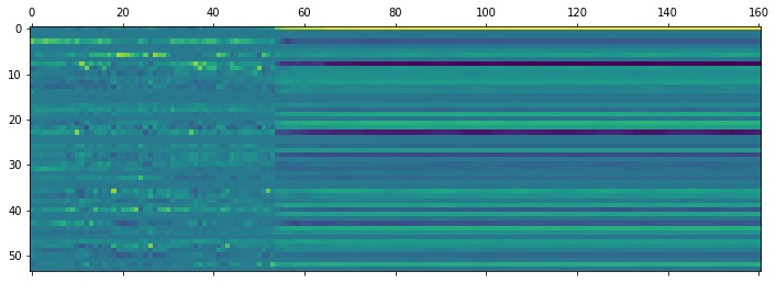
Instead of padding all token list to the same lenght, this will only be done on a per mini-batch basis with the pad_sequences utility from PyTorch. It is worth noting that the pad-sequences will turn a list of tensors into a tensor where the sequence is the first dimension, and batches the second. This is probably because the RNN objects expect this format as it is easier to iterate through the first dimension. For visualization I transpose the tensor.
from torch.nn.utils.rnn import pad_sequence
product_padded = pad_sequence(product_tokens)
plt.matshow(product_padded.numpy().T)
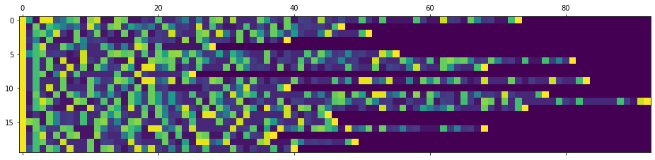
That’s pretty good if the architecture is flexible enough to use variable length minibatches. There’s a lot of computations saved. If we had instead padded all token sequences to the same length, the above mini-batch would be 202 tokens long, thats more than double the lenght that was necessary.
With the tokenizer in place, we can start to look at the datasets. Just the train and validation sets will be used in this simple example.
X_train = data.reactant_ROMol[data.set == "train"]
y_train = data.products_ROMol[data.set == "train"]
X_val = data.reactant_ROMol[data.set == "valid"]
y_val = data.products_ROMol[data.set == "valid"]
A variable to tell where the tensors and models should ultimately be computed can be a good thing to define.
device = torch.device("cuda:0" if torch.cuda.is_available() else "cpu")
print(device)
cuda:0
PyTorch uses datasets to provide the samples. Subclassing the Dataset class allows us to make a specific one that uses the tokenizer to return a list of tensors. They are kept at the cpu and should just be moved to the gpu in the training loop, as all the preprocessing of each mini-batch will be done in parallel on the cpu.
class MolDataset(Dataset):
    def __init__(self, reactants, products, tokenizer, augment):
        self.reactants = reactants
        self.products = products
        self.tokenizer = tokenizer
        self.augment = augment
    def __len__(self):
        return len(self.reactants)
    def __getitem__(self, idx):
        if torch.is_tensor(idx):
            idx = idx.tolist()
        reactants = self.reactants.iloc[idx]
        products = self.products.iloc[idx]
        reactants_tokens = self.tokenizer.tokenize([reactants], augment=self.augment)[0]
        products_tokens = self.tokenizer.tokenize([products], augment=self.augment)[0]

        return reactants_tokens, products_tokens
With the class in place it is possible to instantiate the actual train and validation dataset objects. They’ll provide the tensors when given an index. Augmentation lead to a higher validity but lower accuracy of the prediction. It turns out the sequences of the canonical form are more sequence-wise related than the average pair of augmented SMILES forms, so a lot of preprocessing is necessary to get the right pairs using the Levenshtein distances, more details can be found in the publication: Levenshtein Augmentation Improves Performance of SMILES Based Deep-Learning Synthesis Prediction. For simplicity we will simply use the canonical SMILES in this blog post.
train_dataset = MolDataset(X_train, y_train, tokenizer, augment=False)
val_dataset = MolDataset(X_val, y_val, tokenizer, augment=False)
reactant_tokens, product_tokens = val_dataset[0]
reactant_tokens
    tensor([51,  3,  3,  3,  3,  3,  3,  3, 43,  3, 40, 23,  8,  9, 43, 40,  3,  9,
             6, 36,  6,  6,  6,  6, 40, 33,  6, 48,  6,  6,  6, 40,  3,  3,  3, 40,
            23,  8,  9,  8,  3,  9,  6,  6, 48,  8,  9,  6, 36, 35,  3, 10,  3,  3,
             3, 29, 52])
The pytorch data loaders task is to provide the mini-batches and keep track of shuffling and where we are in the epoch. As we provide both the reactants and products on an item base, the list of (reactant-tensor,product-tensor) will be converted into a list of reactant-tensors and a list of product tensors, before being padded and converted to a joint tensor with the pad_sequence utility. This is done with a small collate_fn, that is provided to the dataloader.
batch_size=120
def collate_fn(r_and_p_list):
    r, p = zip(*r_and_p_list)
    return pad_sequence(r), pad_sequence(p)
train_loader = torch.utils.data.DataLoader(dataset=train_dataset,
                                          batch_size=batch_size,
                                          shuffle=True,
                                          collate_fn=collate_fn,
                                          num_workers=2,
                                          drop_last=True)
val_loader = torch.utils.data.DataLoader(dataset=val_dataset,
                                          batch_size=500,
                                          shuffle=False,
                                          collate_fn=collate_fn,
                                          num_workers=2,
                                          drop_last=True)
Now it’s possible to itereate through the train_loader an get mini-batches of reactants and products. We’ll try a single so that we have something to test with.
for reactants, products in train_loader:
    break
reactants.shape
torch.Size([106, 120])
We’re getting close, now it’s time to define the actual neural network architecture. The nn.Module class is subclassed, the layers are defined in the __init__ and the forward function defines the forward pass of the input tensors through the network. The network is kept very simple, after the tensor of token indexes of the reactants are passed through a learned embedding, a single layer of bidirectional LSTM cells functions as the encoder. The final output of the two directions is summed and is passed through two dense layers that learns to set the initial hidden state C and H of the decoder network. The decoder will read in the product tensors and try to predict the next character, but this shift is defined by an indexing in the actual train loop. The input product tensors are passed through the same embedding layer as the embedding that is useful for the reactants should also be useful for the products. Some dropout layers are added to try and counteract overfitting. I’ve kept the size of the embedding, the number of LSTM cells the same, although they strictly don’t need to be that.
import torch.nn.functional as F
class MolBrain(nn.Module):
    def __init__(self, num_tokens, hidden_size, embedding_size, dropout_rate):
        super(MolBrain, self).__init__() # Inherited from the parent class nn.Module

        self.embedding = nn.Embedding(num_tokens, embedding_size) #Turn tensor of integers into tensor with vectors

        #First layer of the encoder, hidden_size in each direction is half of the hidden_size so that the output is hidden_size
        self.lstm_encoder = nn.LSTM(input_size=embedding_size, hidden_size=hidden_size//2, num_layers=1,
                                    batch_first=False, bidirectional=True)

        #Second layer of the encoder
        self.lstm_encoder_2 = nn.LSTM(input_size=hidden_size, hidden_size=hidden_size//2, num_layers=1,
                                    batch_first=False, bidirectional=True)

        #Transform the output states into a larger size for non-linear transformation
        self.latent_encode = nn.Linear(hidden_size, hidden_size*2)

        #Decode the latent code into the start states for the decoder
        self.h0_decode = nn.Linear(hidden_size*2, hidden_size)
        self.c0_decode = nn.Linear(hidden_size*2, hidden_size)
        self.h0_decode_2 = nn.Linear(hidden_size*2, hidden_size)
        self.c0_decode_2 = nn.Linear(hidden_size*2, hidden_size)

        #First layer of the decoder
        self.lstm_decoder = nn.LSTM(input_size=embedding_size, hidden_size=hidden_size, num_layers=1,
                                    batch_first=False, bidirectional=False)

        #Second layer of the decoder
        self.lstm_decoder_2 = nn.LSTM(input_size=hidden_size, hidden_size=hidden_size, num_layers=1,
                                    batch_first=False, bidirectional=False)

        #fully connected layers for transforming the LSTM output into the probability distribution
        self.fc0 = nn.Linear(hidden_size, hidden_size*2)
        self.fc1 = nn.Linear(hidden_size*2, num_tokens) # Output layer

        #Activation function, dropout and softmax layers
        self.activation = nn.ReLU()
        self.dropout = nn.Dropout(dropout_rate)
        self.softmax = nn.Softmax(dim=2)
    def encode_latent(self, reactants):
        #If batch_size is needed, we can get it like this
        batch_size = reactants.shape[1]

        #Embed the reactants tensor
        reactants = self.embedding(reactants)

        #Pass through the encoder
        lstm_out, (h_n, c_n) = self.lstm_encoder(reactants)
        #print(lstm_out.shape)
        lstm_out2, (h_n_2, c_n_2) = self.lstm_encoder_2(lstm_out)
        #h_n is (num_layers * num_directions, batch, hidden_size)

        #Sum the backward and forward direction last states of the LSTM encoders
        h_n = h_n.sum(axis=0).unsqueeze(0)
        h_n_2 = h_n_2.sum(axis=0).unsqueeze(0)
        #Alternative use internal states
        c_n = c_n.sum(axis=0).unsqueeze(0)
        c_n_2 = c_n_2.sum(axis=0).unsqueeze(0)
        #Concatenate output of both LSTM layers
        #hs = torch.cat([h_n, h_n_2], 2)
        cs = torch.cat([c_n, c_n_2], 2)

        #Non-linear transform of the hs into the latent code
        latent_code = self.latent_encode(cs)
        latent_code = self.dropout(self.activation(latent_code))
        return latent_code

    def latent_to_states(self, latent_code):
        h_0 = self.h0_decode(latent_code)
        c_0 = self.c0_decode(latent_code)
        h_0_2 = self.h0_decode_2(latent_code)
        c_0_2 = self.c0_decode_2(latent_code)
        return (h_0, c_0, h_0_2, c_0_2)
    def decode_states(self, states, product_in):
        h_0, c_0, h_0_2, c_0_2 = states
        #Embed the teachers forcing product input
        product_in = self.embedding(product_in)

        #Pass through the decoder
        out, (h_n, c_n) = self.lstm_decoder(product_in, (h_0, c_0))
        out_2, (h_n_2, c_n_2) = self.lstm_decoder_2(out, (h_0_2, c_0_2))
        #A final dense hidden layer and output the logits for the tokens
        out = self.fc0(out_2)
        out = self.dropout(out)
        out = self.activation(out)
        logits = self.fc1(out)

        return logits, (h_n, c_n, h_n_2, c_n_2)
    def forward(self, reactants, product_in):
        latent_code = self.encode_latent(reactants)
        states = self.latent_to_states(latent_code)
        logits, _ = self.decode_states(states, product_in)
        return logits
We can the number of tokens from the tokenizer, the hidden size is set for 256 and the dropout_rate is also defined. The number of epochs is set and likewise the batch size and learning rate.
num_tokens = tokenizer.dims[1]
hidden_size=256
embedding_size=128
dropout_rate=0.25
epochs = 75
batch_size=128
max_lr = 0.004
model = MolBrain(num_tokens, hidden_size, embedding_size, dropout_rate)
model.to(device)
    MolBrain(
      (embedding): Embedding(54, 128)
      (lstm_encoder): LSTM(128, 128, bidirectional=True)
      (lstm_encoder_2): LSTM(256, 128, bidirectional=True)
      (latent_encode): Linear(in_features=256, out_features=512, bias=True)
      (h0_decode): Linear(in_features=512, out_features=256, bias=True)
      (c0_decode): Linear(in_features=512, out_features=256, bias=True)
      (h0_decode_2): Linear(in_features=512, out_features=256, bias=True)
      (c0_decode_2): Linear(in_features=512, out_features=256, bias=True)
      (lstm_decoder): LSTM(128, 256)
      (lstm_decoder_2): LSTM(256, 256)
      (fc0): Linear(in_features=256, out_features=512, bias=True)
      (fc1): Linear(in_features=512, out_features=54, bias=True)
      (activation): ReLU()
      (dropout): Dropout(p=0.25, inplace=False)
      (softmax): Softmax(dim=2)
    )
A quick test if the forward pass seems to do what it should, by passing the reactants and products batch we got from the dataloader before. The sequence is indexed to be the first to the second last of the tokens. So the first charachter is the “^” start token, and the end-token of the longest sequence is removed.
out = model(reactants.to(device), products[:-1,:].to(device))
out.shape
torch.Size([103, 120, 54])
Good, at least it didn’t crash. The optimizer will be Adam using a little bit of weight decay (L2 regularization) to counteract overfitting.
optimizer = torch.optim.Adam(model.parameters(), weight_decay=1e-5)
The current learning rate is the default.
optimizer.param_groups[0]['lr']
0.001
However, we will use the OneCycle learning rate scheduler. It has a warmup phase that will allows us to use a higher learning rate without instability in the beginning where we have large errors, and a cooldown phase where we get our decision boundary and propability distributions of the output just right.
from torch.optim.lr_scheduler import OneCycleLR
As the learning rate scheduler adjust after each mini-batch, we need to know how many mini-batches we’ll train on. The number of epochs and the length of the train-loader can tell us.
epochs*len(train_loader)
24975
scheduler = OneCycleLR(optimizer=optimizer, max_lr = max_lr, total_steps = epochs*len(train_loader),
                      div_factor=25, final_div_factor=0.08)
Now the learning rate is the start learning rate, which is the max_lr divided by the div_factor.
optimizer.param_groups[0]['lr']
0.00015999999999999999
For fun we’ll make a simple reporter graph that will give a live graph of the training in a jupyter notebook using ipywidgets and some matplotlib.
import ipywidgets
%matplotlib inline
def plot_progress():
    out.clear_output()
    with out:
        print("Epoch %i, Training loss: %0.4F, Validation loss %0.4F, lr %.2E"%(e, train_loss, val_loss, lrs[-1]))
        fig, ax1 = plt.subplots()
        ax1.plot(losses, label="Train loss")
        ax1.plot(val_losses, label="Val loss")
        ax1.set_ylabel("Loss")

        ax1.set_yscale('log')
        ax1.set_xlabel("Epochs")
        ax1.legend(loc=2)
        ax1.set_xlim((0,epochs))
        #Axes 2 for the lr
        ax2 = ax1.twinx()
        ax2.plot(lrs, c="r", label="Learning Rate")
        ax2.tick_params(axis='y', labelcolor="r")
        ax2.set_ylabel("Learning rate")
        ax2.set_yscale('log')
        ax2.legend(loc=0)
        plt.show()
Now for the training!!! First a few collector lists for the losses and the learning rate are initialized and an output area for the live graph is also created. Then we step through the epochs.
In the inner-loop the reactant and product mini-batches are fetched from the train_loader. They are pushed to the device (gpu here). The product in (p_in) is the tokens including the start character, and the p_out is without the start charachter to the end. This right-shift makes the LSTM decoder predict from “^” to e.g. “C”, then from “C” to the third token, and so forth.
The gradient of the optimer is zeroed and the forward pass of the model conducted, which updates the derivatives. The output is transposed to fit the expectations of the loss function, and the loss is calculate with respect to the product output tensor. The loss is then used for the backward pass and gives us the gradients for the optimizer which updates the networks weights.
Finally, the learning rate scheduler updates the learning rate of the optimizer.
After each epoch the model is set in evaluation mode and the loss with respect to the validation set calculated without dropout being active. This is of course done without calculating the gradients and updating the weights. Lastly, the live graph function is called which updates the graph in the “out” ipywidget area.
model.train() #Ensure the network is in "train" mode with dropouts active
losses = []
val_losses = []
lrs = []
out = ipywidgets.Output()
display(out)
for e in range(epochs):
    running_loss = 0
    for reactants, products in tqdm(train_loader, mininterval=1):
        reactant_in = reactants.to(device)
        product_in = products[:-1,:].to(device) #Including starttoken, excluding last
        product_out = products[1:,:].to(device) #Not including start-token

        optimizer.zero_grad() # Initialize the gradients, which will be recorded during the forward pass

        output = model(reactant_in, product_in) #Forward pass of the mini-batch # (batch, sequence - 1, ohe)
        output_t = output.transpose(1,2)

        loss = nn.CrossEntropyLoss()(output_t, product_out)

        loss.backward()
        optimizer.step() # Optimize the weights
        scheduler.step() # Adjust the learning rate

        running_loss += loss.item()
    else:
        with torch.no_grad(): #Don't calculate the gradients
            model.eval() #Evaluation mode
            running_val_loss = 0
            for reactants_val, products_val in val_loader:
                reactant_in = reactants_val.to(device)
                product_in = products_val[:-1,:].to(device)
                product_out = products_val[1:,:].to(device)
                pred_val = model.forward(reactant_in, product_in)
                pred_val = pred_val.transpose(1,2)
                val_loss = nn.CrossEntropyLoss()(pred_val, product_out).item()
                running_val_loss = running_val_loss + val_loss
            val_loss = running_val_loss/len(val_loader)
            model.train() #Put back in train mode

        train_loss = running_loss/len(train_loader)
        losses.append(train_loss)
        val_losses.append(val_loss)
        lrs.append(optimizer.param_groups[0]['lr'])
        plot_progress()
    100%|██████████| 333/333 [00:21<00:00, 15.81it/s]
    100%|██████████| 333/333 [00:20<00:00, 15.92it/s]
    100%|██████████| 333/333 [00:20<00:00, 15.88it/s]
    100%|██████████| 333/333 [00:20<00:00, 15.99it/s]
    100%|██████████| 333/333 [00:20<00:00, 15.92it/s]
    100%|██████████| 333/333 [00:21<00:00, 15.85it/s]
    100%|██████████| 333/333 [00:20<00:00, 16.11it/s]
    100%|██████████| 333/333 [00:20<00:00, 16.01it/s]
    100%|██████████| 333/333 [00:20<00:00, 16.01it/s]
    100%|██████████| 333/333 [00:20<00:00, 15.90it/s]
    100%|██████████| 333/333 [00:20<00:00, 15.99it/s]
    100%|██████████| 333/333 [00:20<00:00, 15.96it/s]
    100%|██████████| 333/333 [00:20<00:00, 15.93it/s]
    100%|██████████| 333/333 [00:20<00:00, 15.87it/s]
    100%|██████████| 333/333 [00:20<00:00, 15.96it/s]
    100%|██████████| 333/333 [00:20<00:00, 15.98it/s]
    100%|██████████| 333/333 [00:20<00:00, 15.91it/s]
    100%|██████████| 333/333 [00:20<00:00, 15.96it/s]
    100%|██████████| 333/333 [00:20<00:00, 15.98it/s]
    100%|██████████| 333/333 [00:20<00:00, 15.95it/s]
    100%|██████████| 333/333 [00:20<00:00, 15.91it/s]
    100%|██████████| 333/333 [00:21<00:00, 15.82it/s]
    100%|██████████| 333/333 [00:20<00:00, 15.90it/s]
    100%|██████████| 333/333 [00:20<00:00, 15.87it/s]
    100%|██████████| 333/333 [00:20<00:00, 15.94it/s]
    100%|██████████| 333/333 [00:20<00:00, 15.93it/s]
    100%|██████████| 333/333 [00:20<00:00, 15.89it/s]
    100%|██████████| 333/333 [00:21<00:00, 15.85it/s]
    100%|██████████| 333/333 [00:20<00:00, 15.90it/s]
    100%|██████████| 333/333 [00:20<00:00, 15.86it/s]
    100%|██████████| 333/333 [00:21<00:00, 15.77it/s]
    100%|██████████| 333/333 [00:20<00:00, 16.02it/s]
    100%|██████████| 333/333 [00:20<00:00, 15.91it/s]
    100%|██████████| 333/333 [00:20<00:00, 15.95it/s]
    100%|██████████| 333/333 [00:20<00:00, 15.88it/s]
    100%|██████████| 333/333 [00:20<00:00, 15.92it/s]
    100%|██████████| 333/333 [00:21<00:00, 15.82it/s]
    100%|██████████| 333/333 [00:20<00:00, 15.87it/s]
    100%|██████████| 333/333 [00:20<00:00, 15.96it/s]
    100%|██████████| 333/333 [00:20<00:00, 15.94it/s]
    100%|██████████| 333/333 [00:21<00:00, 15.85it/s]
    100%|██████████| 333/333 [00:20<00:00, 15.96it/s]
    100%|██████████| 333/333 [00:20<00:00, 16.02it/s]
    100%|██████████| 333/333 [00:21<00:00, 15.85it/s]
    100%|██████████| 333/333 [00:20<00:00, 15.91it/s]
    100%|██████████| 333/333 [00:20<00:00, 15.87it/s]
    100%|██████████| 333/333 [00:20<00:00, 15.97it/s]
    100%|██████████| 333/333 [00:21<00:00, 15.81it/s]
    100%|██████████| 333/333 [00:20<00:00, 15.91it/s]
    100%|██████████| 333/333 [00:20<00:00, 16.10it/s]
    100%|██████████| 333/333 [00:20<00:00, 15.96it/s]
    100%|██████████| 333/333 [00:20<00:00, 15.97it/s]
    100%|██████████| 333/333 [00:21<00:00, 15.75it/s]
    100%|██████████| 333/333 [00:21<00:00, 15.71it/s]
    100%|██████████| 333/333 [00:20<00:00, 15.96it/s]
    100%|██████████| 333/333 [00:20<00:00, 15.99it/s]
    100%|██████████| 333/333 [00:21<00:00, 15.85it/s]
    100%|██████████| 333/333 [00:20<00:00, 15.91it/s]
    100%|██████████| 333/333 [00:20<00:00, 15.94it/s]
    100%|██████████| 333/333 [00:21<00:00, 15.84it/s]
    100%|██████████| 333/333 [00:20<00:00, 15.91it/s]
    100%|██████████| 333/333 [00:21<00:00, 15.77it/s]
    100%|██████████| 333/333 [00:20<00:00, 15.92it/s]
    100%|██████████| 333/333 [00:21<00:00, 15.76it/s]
    100%|██████████| 333/333 [00:20<00:00, 16.00it/s]
    100%|██████████| 333/333 [00:20<00:00, 15.88it/s]
    100%|██████████| 333/333 [00:20<00:00, 15.91it/s]
    100%|██████████| 333/333 [00:21<00:00, 15.74it/s]
    100%|██████████| 333/333 [00:20<00:00, 15.88it/s]
    100%|██████████| 333/333 [00:20<00:00, 15.86it/s]
    100%|██████████| 333/333 [00:20<00:00, 15.90it/s]
    100%|██████████| 333/333 [00:21<00:00, 15.84it/s]
    100%|██████████| 333/333 [00:21<00:00, 15.82it/s]
    100%|██████████| 333/333 [00:21<00:00, 15.84it/s]
    100%|██████████| 333/333 [00:20<00:00, 15.87it/s]
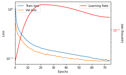
Seems slightly overfit as the train loss suddenty drops in the end, without the test loss changing. But at least the validation loss then converged. Prolonged training with more epochs will give rising validation loss, so maybe the dropout and weight decay are not completely tuned. However, this is probably more or less the best this architecture has to offer. The model and the tokenizer can be pickled for later usage.
import pickle
save_dir = "drive/MyDrive/Colab Notebooks/Reaction_seq2seq_LSTM/"
pickle.dump(model, open(f"{save_dir}seq2seq_molbrain_model.pickle","wb"))
pickle.dump(tokenizer, open(f"{save_dir}seq2seq_molbrain_model_tokenizer.pickle","wb"))
Let’s do a quick test and look at the output.
_ = model.eval()
for reactants, products in val_loader:
    reactants_in = reactants.to(device)
    product_in = products[:-1,:].to(device)
    product_out = products[1:,:].to(device)
    break
reactants_in.shape
torch.Size([165, 500])
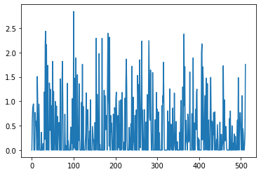
If we predict from the reactant in and product in, what does the output look like? We detach the tensor from the network, pulls to the CPU and converts to numpy array.
i = 0 #Select compound i from validation batch
with torch.no_grad():
  pred = model.forward(reactants_in, product_in)
  pred_cpu = pred[:,i,:].cpu().detach().numpy()
pred_cpu.shape
(161, 54)
plt.matshow(pred_cpu.T)
It’s clear where the sequence stops, and the rest of the prediction is padding.
Greedy sampling simply takes the most probable next charachter with the highest logits, so we can do this fast along the first axis without calculating the softmax along the second axis.
indices = pred_cpu.argmax(axis=1)
indices.shape
(161,)
If we reverse_tokenize the indexes, something that looks like a SMILES string is returned.
smiles = tokenizer.reverse_tokenize(indices.reshape(1,-1), strip=False)
smiles[0]
'CCCCCCCNC(=O)O(C)c1cccc(-c2ccc(CCC(=O)OCCcc2OCCCCl)c1$ '
It seems similar to the target SMILES.
target_smiles= tokenizer.reverse_tokenize(product_out.T, strip=False)
target_smiles[i]
'CCCCCCCNC(=O)N(C)c1cccc(-c2ccc(CCC(=O)OC)cc2OCCCCl)c1$ '
However, we fail to convert it to a molecule object as there are one or more mistakes.
Chem.MolFromSmiles(smiles[0].strip(" $"))
RDKit ERROR: [14:12:27] SMILES Parse Error: extra open parentheses for input: 'CCCCCCCNC(=O)O(C)c1cccc(-c2ccc(CCC(=O)OCCcc2OCCCCl)c1'
This is partly because we see the output from the teacher forced object, where we are not feeding back the prediction to the model for prediction of the next character. So maybe the “mistakes” made above would have been OK, but just a slightlt different SMILES form of the same molecule. Instead, we need to sample the model auto-regressively. First step is to get the latent code from the encoder.
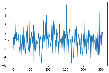
This function allows us to the the latent code for the reactants. It looks like this for this molecule. All information regarding the reactants and possibly what product it should be converted too, are encoded in these numbers. Incomprehensible for me, but the decoder LSTM’s know what to do with the contained information.
latent = model.encode_latent(reactants_in[:,i:i+1])
plt.plot(latent.cpu().detach().numpy().flatten())
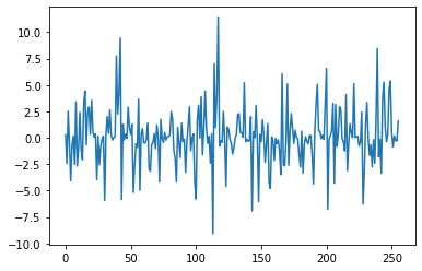
Next, it is possible to calculate the initial states for H and C for the decoder using the relevant layers of the model.
The initial hidden states for the first layer looks like this.
states = model.latent_to_states(latent)
plt.plot(states[0].cpu().detach().numpy().flatten())
print(states[0].shape)
torch.Size([1, 1, 256])
And the initial C state for the first decoder layer:
plt.plot(states[1].cpu().detach().numpy().flatten())
The greedy decode will initialize the decoder with the h0 and C0 states and feed it the start character token index. Then the token with the highest probability is selected and fed back in. The states h_i and c_i are constantly updated and fed back to the network for the next computation. When the stop character is the highest probability the loop will stop, and return the sequence.
def greedy_decode(model, states):
        char = tokenizer._char_to_int["^"]
        last_char = char
        stop_char = tokenizer._char_to_int["$"]
        char = torch.tensor(char, device=device).long().reshape(1,-1) #The first input
        chars = [] #Collect the sampled characters
        for i in range(200):
            out, states = model.decode_states(states, char.reshape(1,-1))
            out = model.softmax(out)
            char = out.argmax() #Sample Greedy and update char
            last_char = char.item()
            if last_char == stop_char:
                break
            chars.append(last_char)

        return chars

smiles = greedy_decode(model, states)
result = tokenizer.reverse_tokenize(np.array([smiles]))
result
    array(['CCCCCCCNC(=O)Oc1cccc(-c2ccc(CCC(=O)OCC)cc2CN(CC)CC)c1'],
          dtype='<U53')
Chem.MolFromSmiles(result[0], sanitize=False)
Lets see if this was the right molecule …
target_smiles= tokenizer.reverse_tokenize(product_out.T)
#target_smiles[i]
print(target_smiles[i])
Chem.MolFromSmiles(target_smiles[i].strip(" $"))
CCCCCCCNC(=O)N(C)c1cccc(-c2ccc(CCC(=O)OC)cc2OCCCCl)c1$
Not quite, but there’s many elements from the molecule that are present, but assembled slightly wrong. It will be interesting to sample some different exampes from the validation set. The latent code can be predicted for all the validation batch of 500.
reactants_in.shape
torch.Size([165, 500])
latent = model.encode_latent(reactants_in)
latent.shape
torch.Size([1, 500, 512])
Likewise the hidden states for the decoder.
states = model.latent_to_states(latent)
states[0].shape
torch.Size([1, 500, 256])
states[1].shape
torch.Size([1, 500, 256])
However, the decode function was not written for operation of batches, so here a simple for-loop is used for this quick test.
results = []
for i in range(500):
    h_in = states[0][:,i:i+1,:]
    c_in = states[1][:,i:i+1,:]
    h_in_2 = states[2][:,i:i+1,:]
    c_in_2 = states[3][:,i:i+1,:]

    chars = greedy_decode(model, (h_in, c_in, h_in_2, c_in_2))
    smiles = tokenizer.reverse_tokenize(np.array([chars]))[0]
    reactant_smiles = tokenizer.reverse_tokenize(reactants.T[i:i+1])[0].strip(" $")
    product_smiles = tokenizer.reverse_tokenize(product_out.T[i:i+1])[0].strip(" $")

    results.append({"product":product_smiles,
                   "reactants":reactant_smiles,
                   "predicted":smiles})
Converting the results to a pandas dataframe and adding the molecules for further analysis
result_data = pd.DataFrame(results)
result_data.head(1)
| product | reactants | predicted | |
|---|---|---|---|
| 0 | CCCCCCCNC(=O)N(C)c1cccc(-c2ccc(CCC(=O)OC)cc2OC… | CCCCCCCNC(=O)N(C)c1cccc(-c2ccc(CCC(=O)OC)cc2O)… | CCCCCCCNC(=O)Oc1cccc(-c2ccc(CCC(=O)OCC)cc2CN(C… |
PandasTools.AddMoleculeColumnToFrame(result_data,'product','product_mol')
PandasTools.AddMoleculeColumnToFrame(result_data,'reactants','reactants_mol')
PandasTools.AddMoleculeColumnToFrame(result_data,'predicted','predicted_mol')
    RDKit ERROR: [14:12:43] Can't kekulize mol.  Unkekulized atoms: 4 5 6 17 19
    RDKit ERROR:
    RDKit ERROR: [14:12:43] Can't kekulize mol.  Unkekulized atoms: 2 3 4 5 6 7
    RDKit ERROR:
    RDKit ERROR: [14:12:43] Can't kekulize mol.  Unkekulized atoms: 7 8 9
    RDKit ERROR:
    RDKit ERROR: [14:12:43] Can't kekulize mol.  Unkekulized atoms: 2 3 4 16 17 18 19 20 37
    RDKit ERROR:
    RDKit ERROR: [14:12:43] Can't kekulize mol.  Unkekulized atoms: 10 11 12 13 14 15 16 17 18
    RDKit ERROR:
    RDKit ERROR: [14:12:43] Can't kekulize mol.  Unkekulized atoms: 16 17 18 19 20 21 22
    RDKit ERROR:
    RDKit ERROR: [14:12:43] Can't kekulize mol.  Unkekulized atoms: 11 12 13 14 31
    RDKit ERROR:
    RDKit ERROR: [14:12:43] Can't kekulize mol.  Unkekulized atoms: 11 12 13 14 24
    RDKit ERROR:
    RDKit ERROR: [14:12:43] Can't kekulize mol.  Unkekulized atoms: 28 29 30 31 33 34 35 36 37
    RDKit ERROR:
    RDKit ERROR: [14:12:43] SMILES Parse Error: unclosed ring for input: 'N#CC1(NC(=O)[C@@H]2CCCC[C@H]2N(Cc2cc(-c3ccc(F)cc3)c(-c3ccccn3)c(S(=O)(=O)C3CC3)s2)CC2)CC1'
    RDKit ERROR: [14:12:43] Can't kekulize mol.  Unkekulized atoms: 14
    RDKit ERROR:
    RDKit ERROR: [14:12:43] SMILES Parse Error: unclosed ring for input: 'COc1ccc2ncc(-c3ccc4c(c3)CC(=O)N4CCC(CCN3C(=O)OCc4cccc5c4s3)C2)n1'
    RDKit ERROR: [14:12:43] Can't kekulize mol.  Unkekulized atoms: 4 5 6 8 20
    RDKit ERROR:
    RDKit ERROR: [14:12:43] Explicit valence for atom # 11 N, 4, is greater than permitted
    RDKit ERROR: [14:12:43] Can't kekulize mol.  Unkekulized atoms: 2 3 41
    RDKit ERROR:
    RDKit ERROR: [14:12:43] Can't kekulize mol.  Unkekulized atoms: 1 2 3 4 59
    RDKit ERROR:
    RDKit ERROR: [14:12:43] Can't kekulize mol.  Unkekulized atoms: 2 3 4 5 6 7 8 17 18 19 20 22 23
    RDKit ERROR:
    RDKit ERROR: [14:12:43] Can't kekulize mol.  Unkekulized atoms: 3 4 5 6 14 16 17
    RDKit ERROR:
    RDKit ERROR: [14:12:43] Can't kekulize mol.  Unkekulized atoms: 1 2 3 4 5 6 7 26 27
    RDKit ERROR:
    RDKit ERROR: [14:12:43] SMILES Parse Error: unclosed ring for input: 'CC(=O)N1CCC(N2CCC[C@H](NC(=O)c3c(CN4CCOCC5)cccc43)CC2)Cc2ncccc21'
    RDKit ERROR: [14:12:43] SMILES Parse Error: unclosed ring for input: 'COc1ccc(C(=O)c2oc3c(C)c(C)cc(C)c3c2c2ccccc23)c1O'
    RDKit ERROR: [14:12:43] Can't kekulize mol.  Unkekulized atoms: 14 15 16 17 18 19 24 25 26 27 28 29 30 31 32
    RDKit ERROR:
    RDKit ERROR: [14:12:43] SMILES Parse Error: unclosed ring for input: 'CN(C)C(=O)c1cc2cnc(Nc3ccc(C(=O)N4CCC[C@@H]5CO)cn4)nc3c(C3CC3)cn2[C@H]1CCO'
    RDKit ERROR: [14:12:43] Can't kekulize mol.  Unkekulized atoms: 13 14 15 16 17 18 20 21 22 23 24 25 26 28 29 30 31
    RDKit ERROR:
    RDKit ERROR: [14:12:43] Can't kekulize mol.  Unkekulized atoms: 2 3 4 5 6 7 8
    RDKit ERROR:
    RDKit ERROR: [14:12:43] Can't kekulize mol.  Unkekulized atoms: 1 2 4 6 7 10 14 20 21
    RDKit ERROR:
    RDKit ERROR: [14:12:43] Can't kekulize mol.  Unkekulized atoms: 4 5 6 7 8 9 10
    RDKit ERROR:
    RDKit ERROR: [14:12:43] Can't kekulize mol.  Unkekulized atoms: 28 29 30 32 47 48 49
    RDKit ERROR:
    RDKit ERROR: [14:12:43] SMILES Parse Error: unclosed ring for input: 'C[C@@H]1CC[C@H]2[C@@H](CC[C@H]3C[C@@H](OC4CCC(O)(c5ccc(-c6cccnn6C6C)cc5)CC4)C=C3)C=C2C1'
    RDKit ERROR: [14:12:43] Can't kekulize mol.  Unkekulized atoms: 5 6 7 23 24
    RDKit ERROR:
    RDKit ERROR: [14:12:43] Can't kekulize mol.  Unkekulized atoms: 3 4 5 6 7 8 13 16 19
    RDKit ERROR:
    RDKit ERROR: [14:12:43] Explicit valence for atom # 23 C, 5, is greater than permitted
    RDKit ERROR: [14:12:43] Can't kekulize mol.  Unkekulized atoms: 14 15 16 17 18
    RDKit ERROR:
    RDKit ERROR: [14:12:43] non-ring atom 13 marked aromatic
    RDKit ERROR: [14:12:43] Can't kekulize mol.  Unkekulized atoms: 4 5 6 35 40
    RDKit ERROR:
    RDKit ERROR: [14:12:43] Can't kekulize mol.  Unkekulized atoms: 6 7 8 9 10 11 20
    RDKit ERROR:
    RDKit ERROR: [14:12:43] Explicit valence for atom # 10 N, 4, is greater than permitted
    RDKit ERROR: [14:12:43] Can't kekulize mol.  Unkekulized atoms: 14 15 17 18 19
    RDKit ERROR:
    RDKit ERROR: [14:12:43] Can't kekulize mol.  Unkekulized atoms: 2 3 4 22 23 24 25 28 29
    RDKit ERROR:
    RDKit ERROR: [14:12:43] Can't kekulize mol.  Unkekulized atoms: 11 12 13 29 30
    RDKit ERROR:
    RDKit ERROR: [14:12:43] Can't kekulize mol.  Unkekulized atoms: 6 7 8 9 10
    RDKit ERROR:
    RDKit ERROR: [14:12:43] SMILES Parse Error: unclosed ring for input: 'CCOCC(=O)OCC(=O)O[C@H]1CC[C@H]2[C@@H]3CC[C@H]4C[C@@]5(C)[C@@H](CO)CC[C@]4(C)[C@H]3C(=O)C[C@]12C'
As it is apparent from the RDKit conversion errors some of the SMILES were malformed. It’s simple to calculate how many percent were invalid.
invalid = (result_data.predicted_mol.isna()).sum() / len(result_data)
invalid
0.084
It’s possible to look at the molecules directly in the dataframe. The predicted products are clearly related to the reactants, but do contain various errors. Swapping of halogens, regioisomers, wrong assembly of substructures and wrong length of alifatic carbon chains seem to be common errors.
result_data[["reactants_mol","product_mol","predicted_mol"]].head(20)
| reactants_mol | product_mol | predicted_mol | |
|---|---|---|---|
| 0 |  |
 |
 |
| 1 |  |
 |
|
| 2 |  |
 |
 |
| 3 |  |
 |
 |
| 4 |  |
 |
 |
| 5 |  |
 |
|
| 6 |  |
 |
 |
| 7 |  |
 |
 |
| 8 |  |
 |
 |
| 9 |  |
 |
 |
| 10 |  |
 |
 |
| 11 |  |
 |
None |
| 12 |  |
 |
 |
| 13 |  |
 |
 |
| 14 |  |
 |
 |
| 15 |  |
 |
|
| 16 |  |
 |
 |
| 17 |  |
 |
 |
| 18 |  |
 |
 |
| 19 |  |
 |
 |
We can compare identity on the molecular level by comparing the canonical SMILES strings.
correct = 0
wrong = 0
invalid = 0
for row in result_data.iterrows():
    try:
        mol = Chem.MolToSmiles(row[1]["product_mol"])
        target = Chem.MolToSmiles(row[1]["predicted_mol"])
        if target == mol:
            correct = correct + 1
        else:
            wrong = wrong + 1
    except:
        invalid = invalid + 1
correct/len(result_data)
0.1
wrong/len(result_data)
0.816
invalid/len(result_data)
0.084
So this model is a near miss. Validity of the SMILES seem to be reasonable good (thanks to teachers forcing), but the accuracy of the prediction is quite low. With beamsearch and more carefull tuning of the hyperparameters it could possibly be improved somewhat, more layers and larger hidden size could maybe also help. But mostly, larger datasets and more complex architectures are needed for this to fly (hint: Transformers). The problem with the LSTMs is that all information has to constantly be encoded in the hidden states and the latent code transferred. This gives a lower fidelity in the reconstruction when there’s no attention mechanisms. However I hope this simple model was instructive in how it can be possible to use sequence based NLP models to handle reaction informatics.
Hello Esben,
I am learning your new lesson by reproducing this work.
When I tried to execute this line “product_tokens = tokenizer.tokenize(data.products_ROMol[0:20])”, I keep receiving an error in this section:
# Convert SMILES to tokens
tokens = torch.tensor([self._char_to_int for c in smiles], dtype=torch.long)
TypeError: an integer is required (got type dict)
I believe that there is something wrong with the type such that it is supposed to produce integers rather than dictionary. Does it relate to the “PandasTools”? I don’t think an error is caused by PandasTools, it is worth a guess
Hi Tommy, thanks for your interest in my blogpost. Unfortunetely WordPress sometimes “eats” part of the code in square brackets as the software interpret it as markup even if it is in a paragraph marked as preformatted. The list comprehension is missing a [c] and instead of building a list of integers using lookups in the dictionary, builds a list of dictionaries, which of course can’t be converted to a torch tensor. The list comprehension should look [self._char_to_int[c] for c in smiles]. I’ll see if I can get wordpress not to remove the code.
Best Regards
Esben
Hello Mr. Bjerrum,
Thank you for clarifying it for me! Because of that, I replaced char_to_int with another function, which also works the same. Because the the “eating words” issue from WordPress, may I ask if it also happens to these lines as well?
“for reactants, products in train_loader:
break
reactants.shape
“.
Overall, it looks like the model’s prediction is very bad here, lower than what I thought.
Those lines are fine. It’s a dirty way to create an iterator and get the first item.
The models performance at this stage is of course 0, as it has not been trained yet. Moreover, the LSTM networks struggle with the fidelity of the prediction, so overall accuracy on the molecular level is low. Transformer networks are much better, check out the next blogpost Transformer for Reaction Informatics – utilizing PyTorch Lightning